Towards the second PR
In the previous post I described the Next Subvolume Method. Once that PR was merged, I wrote an issue outlining what needs to be done next. My next PR will complete the top 6 TODOs on the list. Most importantly, it introduces more comprehensive tests and three optimized CartesianGrid structs.
Improving the tests
The previous PR only tested the NSM on 1D grids, which left room for bugs to go undetected. In this PR I added a way to test pure diffusion on arbitrary graphs. First, given a graph and a hopping rate (probability per time of hopping to a neighboring site) we must contruct the discrete Laplacian matrix . The following function does that.
function discrete_laplacian_from_spatial_system(spatial_system, hopping_rate)
    sites = 1:DiffEqJump.num_sites(spatial_system)
    laplacian = zeros(Int, length(sites), length(sites))
    for site in sites
        laplacian[site,site] = -DiffEqJump.num_neighbors(spatial_system, site)
        for nb in DiffEqJump.neighbors(spatial_system, site)
            laplacian[site, nb] = 1
        end
    end
    laplacian*hopping_rate
end
We now have the system of differential equations , where is the expected number of species at time . The solution is given by , which is computed by the following script.
lap = discrete_laplacian_from_spatial_system(LightGraphs.grid(dims), hopping_rate)
evals, B = eigen(lap) # lap == B*diagm(evals)*B'
Bt = B'
analytic_solution(t) = B*diagm(ℯ.^(t*evals))*Bt * reshape(prob.u0, num_nodes, 1)
A neat fact from linear algebra is that a symmetric matrix is always diagonalizable, and is symmetric. So the procedure above will always work.
By the weak law of large numbers we know that the average of many simulations should converge to the expected value, which is what we test.
Nsims = 10000
rel_tol = 0.01
grids = [DiffEqJump.CartesianGrid1(dims), DiffEqJump.CartesianGrid2(dims), DiffEqJump.CartesianGrid3(dims), LightGraphs.grid(dims)]
for grid in grids
    spatial_jump_prob = JumpProblem(prob, alg, majumps, hopping_constants=hopping_constants, spatial_system=grid, save_positions=(false,false)) #set up the jump problem
    mean_sol = get_mean_sol(spatial_jump_prob, Nsims, tf/num_time_points) # average of 10000 runs
    for (i,t) in enumerate(times)
        local diff = analytic_solution(t) - reshape(mean_sol[i], num_nodes, 1)
        @test abs(sum(diff[1:center_node])/sum(analytic_solution(t)[1:center_node])) < rel_tol
    end
end
Optimizing Cartesian grid
A 3 by 3 Cartesian grid:
| 1 | 4 | 7 |
| 2 | 5 | 8 |
| 3 | 6 | 9 |
A frequent use-case for spatial SSAss is to do simulation on a 1D, 2D or 3D rectangular grid in Euclidean space. For example, we might want be interested in some molecule diffusing on a small patch of a cell's membrane, which is basically a two-dimensional rectangle. While this is a special case of a graph, it is common enough to implement it separately and efficiently. I implemented three versions of a Cartesian grid in utils.jl. The most important function required of a graph or a Cartesian grid is rand_nbr(grid, site), which outputs a random neighbor of site with uniform probability. For an arbitrary graph it is simply
rand_nbr(graph::AbstractGraph, site) = rand(neighbors(graph, site))where neighbors(graph, site) is a pre-computed list of neighbors.
For a Cartesian grid there is no need to pre-compute the list of neighbors for each site because of strong regularity of the neighbor list. For example, in a 2D grid, each site has 4 neighbors (up, down, left, right) except those neighbors that are outside the grid. For example, site 4 has neighbors 1, 7, and 5. In a grid, we would need an array of length to store the list of all neighbors, which is not cache-friendly. So what are the alternatives to pre-computing all neighbors?
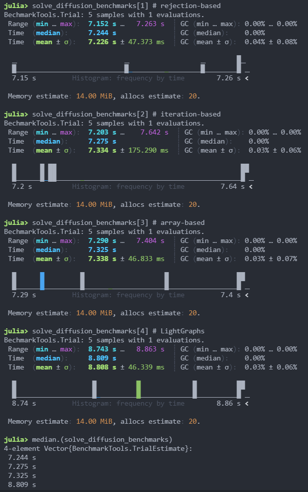
We can rejection-sample a neighbor in the following fashion. Given a site, assume that it has all 4 (or 6 in case of 3D) neighbors and pick a random one. If it is inside the grid, we have our neighbor. Otherwise, do the same thing again. Since most sites have all 4 (6)neighbors, the probability of having to try again is small. This turns out to be the fastest sampling method for large grids, according to my benchmarking.
We can sample a neighbor by iterating. Pre-compute the number of neighbors for each site, and given a site, draw a random number from 1 to the number of neighbors of the site. Then iterate to that neighbor, discarding those potential neighbors that are outside the grid.
In order to find out which method (pre-computing neighbors, rejection-sampling or iteration-sampling) is the fastest I imlpemented three version of a Cartesian grid and benchmarked them. The rejection-sampling method came out to be the winner for larger () grids.
Further work
The next step is to add support of various forms of hopping rates. Currently, the assumption is that hopping rates are of form , where is a species and is a site (i.e. hopping rates depend only on the species and site). Other common forms of hopping rates include , , and . Each of these is a special case of , so implementing this is the priority, but each special case allows for more efficient memory usage and thus better performance.
At the moment there are two data main structures used in spatial simulation: AbstractSpatialSystem and AbstractSpatialRates. The role of the first is to contain all information about the topology (number of sites, number of neighbors for each site, sampling a random neighbor). The role of the second is to contain all information about the current rates of reactions and jumps. In order to improve orthogonality AbstractSpatialRates can be split into AbstractRxRates and AbstractHoppingRates. Depending on the form that hopping or reaction rates take, the user will pass in different objects, making it easy to "assemble" the spatial simulation.