First achievements: Next Subvolume Method

The past two weeks saw me work on my first PR this summer, and it is almost done. I implemented the Next Subvolume Method (Elf and Ehrenberg (2004)), developed an interface for spatial SSAs, which is consistent with the existing interface, and tested the newly implemented SSA.

Spatial SSAs

When simulating spatially non-homogeneous systems the standard approach is to split the domain into small sub-domains (often called sites). Each sub-domain is assumed to be well-mixed. Now there are two types of events/jumps that can happen at each step of the simulation: reactions within a site and diffusions between neighboring sites.

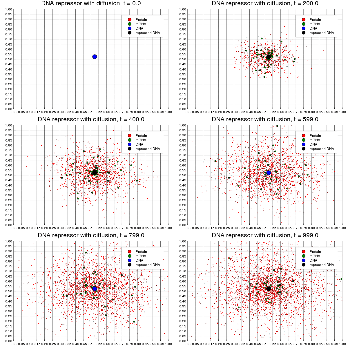
For a concrete example, consider the DNA repressor model (1). It consists of four species: DNA, repressed DNA (DNAR), mRNA, and protein, and six reactions.

\begin{aligned} DNA &\xrightarrow{0.5} mRNA + DNA\\ mRNA &\xrightarrow{0.115} mRNA + P\\ mRNA &\xrightarrow{0.006} ∅\\ P &\xrightarrow{0.001} ∅\\ DNA + P &\xrightarrow{0.025} DNAR\\ DNAR &\xrightarrow{1.0} DNA + P \end{aligned}

The DNA molecule is large, and is assumed not to diffuse. The other two molecules – mRNA and protein – can diffuse around. The result of a simulation of this model is shown in the animation below.

If the mesh size decreases, the number of sites increases quadratically in 2D and cubically in 3D making computational complexity – both theoretical and actual – a concern. The Next Subvolume Method is a stochastic simulation algorithm (SSA) that is easy to implement and is more efficient than a naïve implementation.

Next Subvolume Method

I will describe the Next Subvolume Method (NSM) briefly here. Detailed pseudocode can be found in (Elf and Ehrenberg (2004)).

Each site has its own propensity (probability-per-time) to fire, i.e. to have a reaction or a diffusion happen there. We would like to be able to quickly sample the next site to fire and update its propensity. This can be achieved with a binary minheap, which has $O(1)$ time of getting the minimum element and $O(log\left(\text{number of sites}\right))$ update time. At the beginning of the simulation the propensities of all sites (400 of them in the simulation above) are computed and random firing times are sampled from the exponential distribution with parameter equal to the propensity. The sites are assembled in the minheap, keyed by their sampled firing time. At each step of the simulation the top of the heap is popped off giving the next site to fire. Once the site to fire is chosen we must figure out which jump occurs at this site. It is sampled linearly according to the propensities of the possible reactions and diffusions. After executing the jump at the chosen site, a small number of propensities are recomputed – those, which depend on the occurred jump. The site propensity is also recomputed and the site is put back in the heap.

There are two data structures I implemented to keep track of the relevant information in spatial SSAs: SpatialSystem and SpatialRates. The former contains all information about the topology of the system, while the latter keeps track of all the propensities. I identified the functions needed from each of these and made an interface consisting of these functions, so that any struct that implements these functions can be used in the SSA. This will allow me and other users to implement variants of NSM or other spatial SSAs easily and benchmark different implementations against each other. These are contained in utils.jl.

I spent the most time implementing NSM itself (see nsm.jl). Apart from the functions specific to NSM it contains functions that will be useful for other spatial SSAs, such as update_state!, which updates the current state based on the chosen jump.

Testing & Debugging

Testing and Debugging is an essential part of any coding project. I developed two tests for spatial SSAs: ABC.jl and diffusion.jl. The first one sets up the reversible binding system $A+B \xleftrightarrow{} C$ on a 1D grid with 5 sites and uses non-spatial SSAs to test correctness of the end-state. The second one uses a pure diffusion system on a 1-D grid with 32 sites to test the spatial SSAs against a known analytic solution at eleven time points. The current implementation of NSM passes both tests, which is a good indication of correctness.

Future plans

As one of my CS professors said,

the biggest speed-up your program will ever get is when it starts working.

That's why I focused on getting NSM correct first. Now that the design is done and correctness is established, I can focus on some performance improvements. The biggest one is using @view for slicing to avoid memory allocations. Another is implementing a more efficient SpatialSystem struct. Once I make those two changes and make a few small tweaks per my mentor's advice, this PR will be merged.

In this PR I created a lot of infrastructure that will make implementing and testing spatial SSAs easier. The next spatial SSA to implement is DirectCR + RSSA, i.e. the site is selected with DirectCR and the jump within the site is selected with RSSA. Both are based on rejection sampling, which is an ingenious way to sample stuff fast.

References

Elf, Johan and Ehrenberg, Mäns. “Spontaneous separation of bi-stable biochemical systems into spatial domains of opposite phases”. In: Systems biology 1.2 (2004), pp. 230–236.